Overview of the Field

Understanding Reinforcement Learning Categories is a Must. Reinforcement Learning (RL) spans a wide range of algorithms, each based on different assumptions, optimization principles, and feedback structures. Unlike supervised learning, the diversity of RL approaches—each requiring different theory, tools, and implementation strategies—makes the learning curve steep but rewarding.

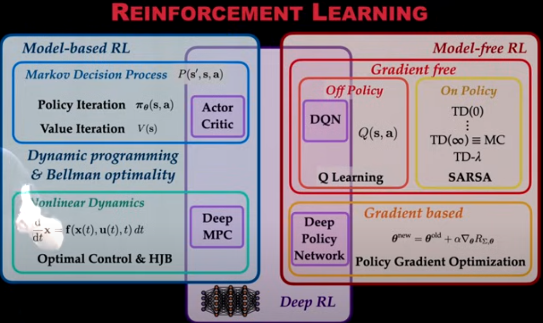
Model-Based vs Model-Free: Availability of Transitions. A core distinction in RL is whether the transition dynamics—represented as $P(s' \mid s, a)$, the probability of ending up in state $s'$ after taking action $a$ in state $s$—are known. In model-based RL (aka DP settings), these dynamics are known or learned and explicitly used to plan optimal behavior. In model-free RL (aka RL settings), we assume no access to this underlying probability, which reflects most real-world situations.

Model-Free RL: Learning Without Transition Knowledge. When we don’t know $P(s' \mid s, a)$, we resort to model-free methods, which learn from direct interaction. These approaches can be further divided into:

1. Gradient-Free Methods, where updates are not derived from explicit gradients.
   • Off-Policy methods (e.g., Q-learning, DQN) learn an optimal policy (action determiner) from data generated by a different behavior policy, allowing better exploration.
   • On-Policy methods (e.g., SARSA, TD learning) learn from and about the same policy, often with more stable but sample-inefficient updates.
2. Gradient-Based Methods, such as Policy Gradient approaches, optimize expected cumulative reward via gradient ascent in the parameter space of a policy network.

Deep RL: A Revolution in Expressiveness. Deep Reinforcement Learning integrates deep neural networks with RL algorithms to handle high-dimensional state and action spaces. Deep RL enable breakthroughs in games (e.g., Atari, Go), robotics, and complex control systems. Deep RL also blurs traditional boundaries, DQNs bring deep learning to value-based methods, while Actor-Critic methods combine policy gradients and value estimation. This integration brings power, but also introduces stability and sample efficiency challenges.

Problem Formulation: Markov Decision Process

This section is a personal revision on ^{[zulfikar2025mdp]} that summarized a week lecture at University of Indonesia Machine Reinforcement Learning by Vektor Dewanto.

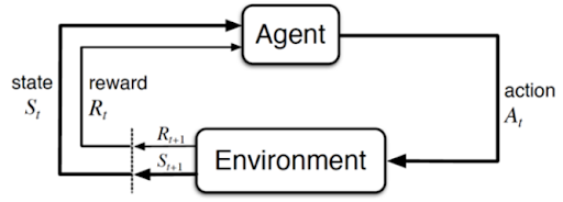
Formal Definition of MDP. The Markov Decision Process (MDP) is a foundational framework used across disciplines—from AI and control theory to economics and operations research. An MDP is defined as the tuple $M = (\mathcal S, \mathcal A, \mathcal T , \dot p, p, r)$, where:

• $\mathcal S$ is the state set, $S = \{s^0, s^1, \dots, s^{\vert\mathcal S\vert}\}$
• $\mathcal A$ is the action set, $A = \{a^0, a^1, \dots, a^{\vert\mathcal A\vert}\}$
• $\mathcal T$ is the time set, $\mathcal T=\{0, 1, 2, \dots\}$, usually people skip this because mostly we only deals with discrete time
• $\dot p: \mathcal S\to [0, 1]$ is the initial state distribution, $\dot p(s)$ probability of starting at a $s$.
• $p:\mathcal S\times\mathcal A\times\mathcal S\to[0,1]$ is the transition function, defined as $p(s'\mid s, a)$, probability of ends in $s'$ given doing action $a$ in $s$
• $r(s, a)$ is the reward function, specifying the expected reward received for taking action $a$ in state $s$. Other form such $r(s'\mid s, a)$ is also possible and could easily converted by marginalization.

Remember that $s^0$ represent state 0, $s_1^0$ represent state 0 at time $t=1$.

Lets Assume Stationary MDPs for Simplicity. In this setting, the state and action sets remain unchanged over time, and our goal is to find a stationary optimal policy. Formally, this means. State space, Action space, transition probability, and reward function is independent of time.

This relaxation could be imagine in chess as, the available actions for any board configuration never change, which simplifies modeling. In contrast, non-stationary MDPs allow these components to vary over time reflects many real-world problem.

Assuming Infinite Horizon and Discrete Time. In addition to stationarity, we often assume an infinite time horizon (i.e., the agent interacts with the environment indefinitely) and discrete time steps. Finite-horizon MDPs are also studied especially in planning problems, but often lead to time-dependent policies. We also assume finite state and action spaces, which enables representations in finite computer’s memory and guarantees convergence.

Markovian: The Markov Assumption on Time Dependency. A core assumption of MDPs is the Markov property, which states that the future state depends only on the current state and action, not on the entire history. This simplifies the transition function to:

rather than

This also often called the first-order Markov assumption. While real-world scenarios often violate this assumption, we either redefine the state to be more informative or use memory-based models (e.g., RNNs in Deep RL) when necessary.

MDP Visual Interpretation. A helpful intuition for this is shown in the diagram below. The agent transitions between various states like “Wake Up”, “Netflix”, “Code & Debug”, and “Deploy”, receiving different rewards depending on its action.

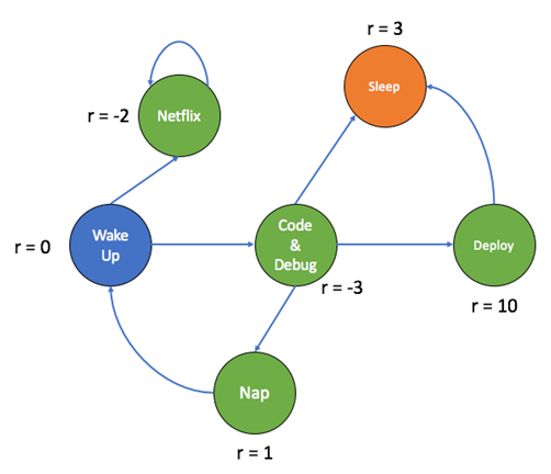
This environment is Markovian: the next state and reward depend only on the current state and action—not on how the agent reached that state. For example, regardless of whether the agent arrived at “Code & Debug” from “Nap” or “Wake Up”, the outcome of choosing “Sleep” will always transition to “Sleep” with a reward of 3.

Policy: The Solution to the MDP. Policy $\pi:\mathcal S\times \mathcal A\to[0, 1]$ defines the agent’s behavior by specifying the probability of choosing each action in each state.

There are two main classes of policies:

1. $\prod_{SR}:$ Represent set of Stationary Randomized/Stochastic policies.
2. $\prod_{SD}:$ Represent set of Stationary Deterministic policies, one action with probability 1, will always be chosen.

A deterministic policy $\pi_{SD}\in\prod_{SD}:\mathcal S\to\mathcal A$ maps single state to single action. It can be viewed as a special case of stochastic policy.

Showing that $\prod_{SD}\subset\prod_{SR}$

Matrix Representation of a Policy. A policy can also be represented as a matrix, where each row corresponds to a state and each column corresponds to an action:

We see that in ith-row, $\pi(\cdot, s^i)$, represent action distribution at state $s^i$, the best action is the maximum among this rows. Please also note that sum over actions must be one $\sum_a \pi(a\mid s)=1$.

Markov Chain: Unique Action MDP. Every MDP with a fixed policy $\pi$ induces a Markov Chain (MC). A Markov Chain is an MDP where each state has a unique action. Because $p(s'\mid s, a)$ and we fix $\pi$, $p(s'\mid s, \pi(s)):\mathcal S\times\mathcal S\to[0, 1]$ could be derived called stochastic transition matrix or one-step state-transition matrix denoted as $P\in R^{\vert\mathcal S\vert\times\vert\mathcal S\vert}$ matrix. Formally

$P_{ij}$ describes the probability of ending at $s^j$ given current state $s^i$.

$P$ is stochastic meaning that

1. Probability entries $0\le P_{ij}\le 1$
2. $\sum_j P_{ij} = 1$, we will always ended up in one of state $s^j$ given current state $s^i$.

K-th Step Transitions. Given Markov Chain (fixed policy), the probability of ending at time k for all states $s_k$ could be computed as

$P^k_{ij}$ now represent the probability of starting (at $t=0$) at $s_i$ and ended up in $s_j$.

State Classification in Markov Chain. Knowing class of a markov chain, we could assure the convergence of an algorithm. In Markov Chains (MC), states can be classified into two main categories:

1. Recurrent: If the probability of returning to s from s is 1. This means that the state will be visited infinitely many times.
2. Transient: If there is a non-zero probability of never returning to s. This means that the state might be left.

Markov Chains Classification. Some theorem will be based on implication of some markov chains class.

1. Recurrent Markov Chain: All states are recurrent, meaning that from any state it is possible to return to that state eventually. There are no transient states in a recurrent Markov Chain. EXAMPLE

2. Unichain Markov Chain: Contains a single recurrent class and possibly some transient states. A recurrent class is a set of states where each state can be reached from any other state within the class, and once entered, the process cannot leave the class. Transient states are those that, once left, cannot be returned to. EXAMPLE

3. Multichain Markov Chain: Contains more than one recurrent class. Each recurrent class is a set of states where each state can be reached from any other state within the class, and once entered, the process cannot leave the class. There may also be transient states that do not belong to any recurrent class. EXAMPLE

Theorem. In Finite MDP, there exists at least one chain.. We classify MDPs as follows:

• Unichain MDP: All induced MCs are unichain.
• Multichain MDP: At least one induced MC is multichain.

Markov Chains Limiting State Transition Matrix P. Denote $P_\pi^\star$ the limiting state transition matrix or converged transition after time.

Since computers cannot compute indefinitely until reaching infinity, we need practical methods to approximate $P_\pi^\star$. Here are two common approaches:

1. Iterative method, we enumerate $k$ and stop for predefined constant or comparing converge tollerance $\Vert P^k-P^{k-1}\Vert_c < \epsilon$, for preference matrix norm $c$ and real threshold $\epsilon$.
2. Close form solution,

with contraint of $P_\pi^\star$ is a stochastic matrix i.e

Theorem. In Unichain Markov Chains, all rows of the limiting state transition matrix $P_\pi^\star$ are identical

Then matrix $P_\pi^\star$ could be represented by single vector $p_\pi^\star$ that satisfy linear system of equations.

Because it is an overdetermined equation, the trick is to

1. Replace the last row of $(P-I)^T$ with $[1\;1\;\dots\;1]$ and store it in matrix $A$.
2. Replace the corresponding entry on the right-hand side (which was originally a zero vector) with 1.
3. Solve the modified system to get the $p_\pi^\star$:

Optimality Criteria and Optimal Policies is the solution for Markov Reward Process (MRP)., MRP is a Markov Chain with an addition to transitioning between states based on a probability distribution, each state also has an associated reward. We need to measure with respect to some optimality criterion denote by $v(\pi, s)$. We parameterize startign state $s$ since starting state will sure affect the quality, more general form could easily derive from marginalizing over initial state distribution, $\mathbb E_{s\sim\dot p}v(\pi, s)$. We then could define the optimal policy is the one that maximize value function $v$.

Theorem. In a finite MDP, an optimal deterministic policy $\pi\in\prod_{SD}$ exists. This means we could reduce the solution search into $\prod_{SD}$ domain which is finite, hence a brute force solution will exists with time complexity of $O(\vert\mathcal S\vert^{\vert\mathcal A\vert})$ (remember that deterministic policy is a function of state to action, we will generate every possible action in every possible state).

Kind of reward value function $v$. Note that all these value function is a function of policy and states. Given fixed policy $\pi$, the form of $v$ is actually a vector of size $\vert\mathcal S\vert$. Optimal policy is based on which value function (optimal criterion) is used.

• Total Value Function $v_{total}$.

Using this, as $t\to\infty$, $v_{total}(\pi, s)\to\infty$ which is unusable in infinite horizon MDP.

• Average Reward Function $v_g$.

This average reward can be calculated using these closed form formula obtained from converge transition probability along with the states reward.

• Discounted Reward $v_\gamma$

The discount factor $\gamma$ ensures convergence by weighting future rewards less as they are further into the future.

• Bias Reward $v_b$

The summation term represents the immediate reward $r$ and $v_g(\pi)$ represents the long-term reward. Thus, their difference can be interpreted as a measure of bias. Derived from the Bellman Average Reward Evaluation Equation (BEE) that will be explained in the following paragraphs.

Theorem. In a unichain Markov Chain, all average reward for different state is the same.

This means that $v_g(s)$ does not depend on the initial state $\dot p$, so we only need to compute $v_g(s^0)$ once then define $\vec v_g = v_g(s^0) \cdot \vec 1$

Form of Reward Function. Take a note that all these reward assume fixed policy $\pi$. And their form is using usual convention, stacking states as the first dimension.

• State action state general form

• State action form

• State based form

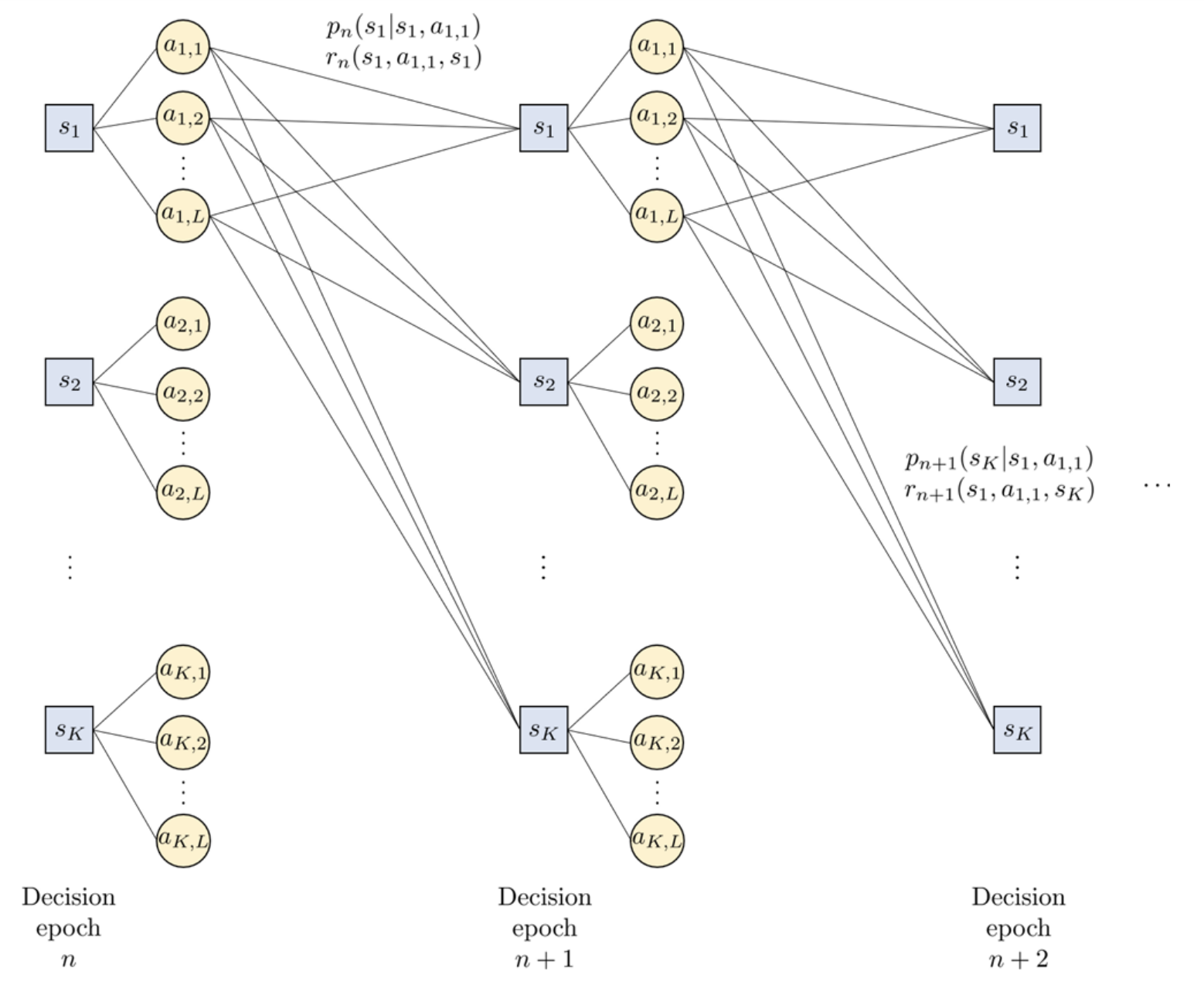
Best visualization for MDP. MDP intuitively could be imagine as a directred acyclic graph with an edge represent possibility.

Bellman Evaluation and Bellman Optimal Equation

Bellman Average Reward Evaluation Equation (BEE). Fundamental equation, the idea is to express immediate and future reward in one equation.

However, there are $\vert S\vert + 1$ unknowns with $\vert S\vert$ number of equations ($\vert S\vert$ of $v_b(\pi, s)$ (one for each state) and single unknown $v_g(\pi)$). This forms an under-determined Linear Equations that will be solved later in following paragraphs.

Making Under-Determined BEE Well-Determine. To solve the under-determined Bellman Average Reward Evaluation Equation (BEE) System of Linear Equations (SLE), we introduce an additional constraint by setting the bias of a reference state to zero.

1. Choose a reference state, say $s^0$, and set its bias to zero: $v_b(\pi, s^0) = 0$
2. Rewrite the formula

Closed-form Solution for $v_b(\pi)$. Remember that $v_g(\pi)=P_\pi^\star \vec r_\pi$. Using this definition, we could manipulate in matrix form then solve it directly.

Note that $H_\pi$ is not a stochastic matrix anymore.The last expression is derive using special case that $P_\pi^\star$ is a fixed point, this implies $(I−A)^{−1}(I−B)=(I−A+B)^{−1}−B$. Trust me you don’t want to see the proof, its really specific. I accept and trust this work from our ancesstor completely without any question. Ask gpt in case you need, he’s capable of deriving this.

Bellman Optimality Equation (BOE). Fundamental concept, it describes the relationship between the value of a state under an optimal policy and the expected return from that state. Optimality condition ensures the equation holds only to the optimal policy, denoted as $\pi^\star$. It is written as

To derive the optimal policy $\pi^\star$, we first obtain optimal $v_b^\star$ and then greedily act wrt the righthand side (RHS) of BOE. Although there may be multiple optimal policies $\pi^\star$, there exists only a single optimal $v_g^\star$ and a single optimal $v_b^\star$.

BOE vs BEE.

1. Applicability: BEE applies to all policies, whereas BOE applies only to the optimal policy.
2. Action Selection: BEE computes the expectation over actions taken by a given policy ($\mathbb E_{a\sim\pi}(\cdot\mid s)$), while BOE selects actions that maximize the expected value ($\max_{a\in\mathcal A}$).
3. Linearity: BEE is a linear equation because it averages over policy actions, whereas BOE is non-linear due to the maximization operator.
4. Value Function Properties: BEE helps evaluate a policy’s value but does not necessarily lead to optimality. In contrast, BOE guarantees that the resulting value function is optimal when solved.

State Action Value Function

The Concept of State Action Value Function $q$. In model-free (RL settings), we don’t know the transition probability $p(s'\mid s, a)$, thus we introduce state action bias (aka state action) $q_b(\pi, s, a)=q_b^\pi(s, a)$ that could eliminate the need for transition probability.

BOE on State Action Value ($q_b$). The optimal action value function satisfies the equation:

Thus the optimal policy can be derived as.

Benefits of BOE for Action Values $q$ over State Values $v$.

1. The optimal policy $\pi^\star(s)$ is greedy with respect to $q_b(s, \cdot)$
2. $q_b$ incorporates the effects of $p(\cdot\mid s, a), r(s, a)$, and $v_b$ without estimating them separately --- crucial since $p$ and $r$ are unknown in the RL settings.

Closed-Form Solution for $q_b^\pi$. We start from the actual definition of action values $q$.

$Q_\gamma$-Learning for Discounted Optimality. Where we use

Alternatively

$r(s, a)+\gamma\max_{a'\in\mathcal A}[\hat q_\gamma^k(s', a')]$ forms the Right-Hand Side (RHS) of the Bellman Optimality Equation (BOE $\gamma$ ) applied to $q_\gamma$.

Convergence criteria for $Q_\gamma$-Learning. Ideally, under the Bellman Optimality Equation (BOE $\gamma$), the difference between the RHS and LHS should be zero upon convergence. Mathematically, this can be expressed as:

Inexact Policy Evaluation

Inexact Policy Evaluation, avoiding the needs for transition probability. In DP setting, we can exactly evaluate a policy via $v_x(\pi, s)$ for arbitrar optimality criterion $x$. However, in RL settings, we have no access in transition probability $P$ and reward scheme $R$. Another problem is that tabular DP method require enumeration of state (or state-action) values which is infeasible for massive large state spaces.

Function Approximation. We approximate value function that can be classify into two categories, parametric and non-parametric.

Parametric Function Approximation. Fixed and finite number of parameters adjusted during learning process. Parametric can simply be broken down into Linear Function (in terms of parameter) and Non-linear Function (Decision Tree and Neural Network).

Non-Parametric Function Approximation. No fixed number of parameters, the complexity grows with the amount of data (KNN, Kernel Methods).

Linear Function Approximation. We define value function $\hat v(s;\vec w)$ as a linear function to approximate $v(s)$. We define feature vector $\vec f(s)\in R^n$ and parameter vector $\vec w\in R^n$.

Where $\vec v\in R^{\vert\mathcal S\vert \times 1}, F\in R^{\vert\mathcal S\vert \times dim(\vec w)}.$ We then learn moving into optimization problem to find $\vec w$ by using optimality criterion $e(\vec w)$.

Where the optimiality criterion $e(\vec w)$ could be mean squared (MS) or projected Bellman (PB).

Linear Function Approximation with (Weighted) Mean Squared Error. We would have $p^\star(s)$ a stationary distribution over states that assigns a weight to each state with a motivation that some states will be visited more often than others. We define weighted mean squared error as

In discrete state spaces, we can expand the expectation and write it down as:

Where $D_{p^\star}$ is a diagonal matrix with $p^\star(s)$ on the diagonal.

To obtain optimal $w^\star$ that minimize MSE, we can use gradient descent.

Approximation of true $v(s)$ in RL settings. Since there are no training data (i.e true $v(s)$ is also unknown), we approximate this using TD or Monte Carlo (MC). We approximate using

This involves the approximation of $\hat v(s; w)$, hence it’s bootstrapping (i.e using an estimation of a value to estimate another one). Because it is an expectation, it is sampling-friendly (i.e using sample of single interaction (s, a, r′, s′) to get the expectation approximation)

Inexact Policy Iteration

Policy Iteration with a Parametric Approach. Since in policy iteration there are two main components, policy evaluation and policy improvement, we could divide the approximation separately.

Approximate Policy Evaluation. We approximate $V^\pi$ or $Q^\pi$ depending which one we adopt. We define finite fixed parameter $w\in R^n$, thus $\hat V(s; w), \hat Q(s, a; w).$ The goal is to minimize error with the true value through similar processes, MSE or TD error. Sometimes we assume linear function approximation such that

Where $\phi(s)\in R^n$ is a feature vector. Pretty identical to Inexact Value Iteration. Sometimes $n=\vert\mathcal S\vert$ becoming a one-hot vector.

Approximate Policy Improvement. Once we have sufficient accurate $\hat V(s)$ or $\hat Q(s, a)$, we perform policy improvement. We update $\pi$ (potentially parameterized to be $\pi(s; w')$). In some scenarios, we might select an action a that maximizes $\hat Q(s, a; w)$ to yield a deterministic policy.

Identical process, error minimization through optimization. Both then define error criterion then optimize using gradient descent. Identical to Indexact Value Iteration and regular Machine Learning framework.

Value Approximation Criterion : Bellman Error and Projected Bellman Error

Above section explain the usage of MSE. Here we will explain the usage of PB. Here we will revisit Bellman Equation, defining bellman error, and then the solution proposed called Projected Bellman Error.

Bellman Equation revisit. The Bellman equation for a value function $v$ can be written in the form

Bellman error measures how well a candidate value function $v$ satisfies the Bellman equation. Basically the difference between approximated $\hat v(s)$ and the true $v(s)$.

When the Bellman error is zero for all states, $v$ exactly satisfies the Bellman equation.

Projected Bellman Error (PBE). Using BEE error, $v$ may lie in a restricted function space (e.g $v$ cannot be represented by $\hat v$ as an implication that we assume $\hat v$ is linear but actual $v$ is not for example). Hence, we cannot always solve in exact, we use projection operator $\Pi$ into our parameter space. Projected bellman error defined as

Where $\mathbb Bv$ is the Bellman operator. We project bellman operation $\mathbb Bv$ into our parameter space $\vec w$.

Minimizing the PBE is a common strategy in methods such as LSTD, where we seek a parameterized value function $\hat v(w)$ that is as close as possible (in a projected sense) to the Bellman update.

How to perform projection $\Pi$. Suppose we have feature matrix $F\in R^{\vert\mathcal S\vert\times k}$ and diagonal weighting $D_{p^\star}\in R^{\vert\mathcal S\vert\times\vert\mathcal S\vert}.$ Each row in $F$ is a feature vector $f(s)^T\in R^k$ with diagonal in $D_{p^\star}$ represent stationary distribution over states. We wish to define a projection

where $\text{Col}(F)$ is the column space spanned by $F$. The projection is taken under the $\ell_2$-norm weighted by $D_{p^\star}$ denoted as

Formally, for any vector $v\in\mathbb R^{\vert S\vert}$, we want to satisfy

Since $x\in \text{Col}(F)$ can be represented as $x=Fw$ for some $w\in R^k$, the problem becomes

This becomes a least squares problem, and the solution is given by

The optimal projection then become

Deriving $w^\star$ to Minimize Projected Bellman Error (PBE). Above is general projection formula if we want to project $v$ into $\text{Col}(F)$. Now we want to project bellman operator on $v$ ($\mathbb B v$).

Utilizing PBE Norm for Precise Objective. We want PBE $=\Pi[\mathbb Bv]- v = \vec 0$, since PBE is a vector, we would need to turn into scalar for optimization which we will use norm. Usually PBE = $\vec 0$ is impossible, we want to be as close as $\vec 0$ as possible. Weighted $\ell_2$ norm could be used.

Full formula for $e_{PB}$.

Under suitable assumption, invertibility of $\{F^TD_{p^\star}(I-P')F\}^{-1}$, we could derive the closed form formuka (well known LSTD solution). It also could be solved using least square.

Main advantage, we do not need the true value function $v$. From these, we can construct the Bellman operator $\mathbb B$ (or an empirical version of it) and compare $\mathbb Bv$ to $v$. This approach is stable because it relies on the self-consistency property of the Bellman equation rather than on direct knowledge of true $v^\star$.

Connection with TD Error. Methods like Temporal Difference (TD) learning effectively estimate the Bellman error incrementally. A TD update can be viewed as trying to drive the quantity

to zero over time, which corresponds to making $v$ satisfy the Bellman equation in expectation.

Value Approximation : Building Matrix $X$ Encoding Transition and Stationary Distribution in RL settings

Another technique for linear approximation of value function, Encoding Transition and Stationary Distribution. We will define $f(s)$ as a feature vector for state $s$, $p^\star(s)$ and $p(s'\mid s)$ stationary distribution and transition probability respectively. We will ended up as simple as solving System of linear equations $Xw=y$ later on.

Intuition of X. We want to build $X$ that encode effect of transition.

We would like to encode the LHS of the above bellman equation.

Direct Definition of $X$. One way is to sum over all states $s$ and possible next statets $s'$ through outer product.

Note that $f(s)f(s)$ is an outer product that form matrix, $f(s)f(s)^T$, that capture pairwise interactions in feature vector. Lets define feature matrix $F\in R^{\vert\mathcal S\vert\times k}=[f(s)^T]_s$ as a matrix of feature vectors. Then we could write $X$ as :